1. Introduction.
2. Study Questions.
3. Analysis to answer the raised questions.
   • What are the most common chest pain types?.
   • Male vs female distribution and whether gender has any significance when developing heart disease.
   • How frequently does exercise-induced angina occur?.
   • Numerical feature distributions.
   • Correlation & relationship analysis.
   • Feature engineering (prep for Machine learning)
   • Modelling the dataset
4. Limitations & Future Work.
5. Future Work.
   • Final Reflection.
6. Notebook (Python)

Introduction

According to the World Health Organisation, cardiovascular disease is one of the leading causes of death, taking an estimated 19.8 million people a year globally in 2022 [1]. This estimate represents approximately 32% of all global deaths. Because of the difficulty involved in diagnosing cardiovascular disease, they have become a silent killer. Researchers have, over time, identified traits that are indicators of potential cardiovascular disease. In this study, data gathered on these traits will be analysed, and machine learning will be used to identify the presence of cardiovascular disease. The dataset that is analysed contains 14 features/traits, and they are:

Features/Traits	Description
Age	Age of the patient (in years)
Sex	Gender of patient (1 = Male, 0 = Female)
Chest pain type	Type of chest pain: 1 = Typical angina2 = Atypical angina3 = non-anginal pain4 = Asymptomatic
BP	Resting blood pressure (mm Hg)
Cholesterol	Serum cholesterol level (mg/dL)
FBS over 120	Fasting blood sugar > 120 mg/dL (1 = True, 0 = False)
EKG results	Resting electrocardiogram results: 0 = Normal1 = ST-T wave abnormality2 = Left ventricular hypertrophy
Max HR	Maximum heart rate achieved
Exercise angina	Exercise-induced angina (1 = Yes, 0 = No)
ST depression	ST depression induced by exercise relative to rest
Slope of ST	Slope of the peak exercise ST segment
Number of vessels fluro	Number of major vessels (0-3) colored by fluoroscopy
Thallium	Thallium stress test result (categorical medical indicator)
Heart Disease	Target Variable: Presence = heart disease detectedAbsence = no heart disease

Study Questions 

What I want to do with this study is answer the following questions:

1. What are the most common chest pain types?
2. Male vs female distribution and whether gender has any significance when developing heart disease.
3. How frequently does exercise-induced angina occur?
4. Numerical feature distributions. 
5.  Correlation & relationship analysis
6. Feature engineering (prep for Machine learning)
   1. Bin age (young/middle/old)
   1. Identify the best model for the dataset
   1. Normalise numeric features (This will be based on the model identified as the best for this dataset)
7. Modelling the dataset.
8. Limitations and future works.
9. Final reflection

Before I dive into answering the above questions, an initial exploratory data analysis has been done on the dataset and here are my findings:

Type of Analysis	Results
Missing data	None of the features/ traits has a missing value.
Data points/rows	The dataset contains 63,000 data points
Descriptive statistics (numerical features/traits)	From the descriptive statistics, none of the traits appears to have extreme outliers given the closeness of the mean and median. The mean and median appear to show normally distributed data. This will be verified using a histogram.
Categorical Vs Numerical	There are nine categorical features and five numerical features.

Analysis to answer the raised questions

1.       What are the most common chest pain types?

Based on the dataset shown in Figure 1, the most common type of chest pain is asymptomatic, accounting for 52.25% of cases. This is followed by non-anginal pain, accounting for 31.31% of reported cases.

Figure 1: Percentage Distribution of Chest

When chest pain type is analysed by gender, differences become apparent. Among males, asymptomatic chest pain is the most frequently reported type, comprising 59.25% of cases. In contrast, females most commonly report non-anginal chest pain.

Figure 2: Percentage distribution of chest pain type within each sex

2.       Male vs female distribution and whether gender has any significance when developing heart disease

As shown in Figure 3, the dataset contains a higher proportion of males (71.47%) compared to females (28.53%).

Figure 3: Percentage distribution of sex (Male vs Female)

To determine whether gender is associated with the development of heart disease, a chi-square test of independence was conducted, as both gender and heart disease status are categorical variables.

The results of the test indicate a statistically significant association between gender and heart disease (p < 0.05). Therefore, we reject the null hypothesis of independence and conclude that gender and heart disease status are significantly associated in this dataset (see Figure 4).

Figure 4: Chi-square test of independence

3.       How frequently does exercise-induced angina occur?

As shown in Figure 3, the dataset contains a higher proportion of non-exercise-induced angina (72.63%) compared to exercise-induced angina (27.37%).

Figure 5: Percentage distribution of Exercise-induced angina

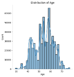
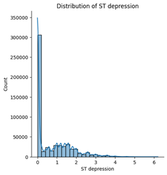
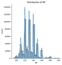
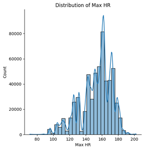
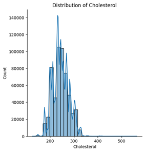
4.       Numerical feature distributions

Among the five numerical features, age, blood pressure (BP), and cholesterol appear to follow an approximately normal distribution. However, ST depression exhibits a right-skewed distribution, whereas maximum heart rate (Max HR) shows a left-skewed distribution (see Figures below).

5.       Correlation & relationship analysis

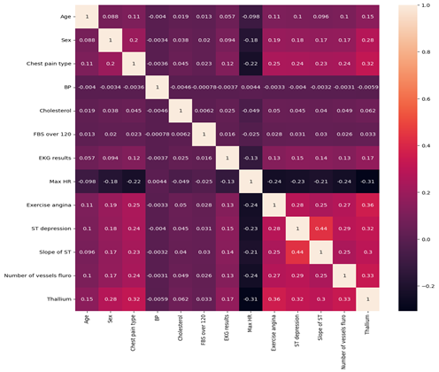
Figure 6: Correlation Matrix

Figure 6 presents the correlation matrix showing the strength and direction of linear relationships between the clinical variables in the dataset.

Overall Observations

Most variables show weak to moderate correlations, indicating that no two predictors are excessively strongly correlated. This suggests a low risk of multicollinearity, which is beneficial for predictive modelling.

Correlation values range from approximately -0.31 to 0.44, indicating generally moderate relationships at most.

Strongest Positive Correlations

The strongest positive relationship observed is:

• ST depression and Slope of ST (r = 0.44)
  This moderate positive correlation suggests that greater ST depression is associated with changes in the slope of the ST segment. Clinically, this is expected, as both variables relate to ECG changes during exercise stress testing.

Other notable positive correlations include:

• Exercise angina and Thallium (r = 0.36)
• Number of vessels fluoroscopy and Thallium (r = 0.33)
• Chest pain type and Thallium (r = 0.32)
• ST depression and Thallium (r = 0.32)

These relationships indicate that imaging results (Thallium test) and exercise-induced symptoms are moderately associated with other markers of cardiac dysfunction.

Strongest Negative Correlations

The strongest negative relationship observed is:

• Max Heart Rate and Thallium (r = -0.31)

This suggests that patients with abnormal Thallium test results tend to achieve lower maximum heart rates during testing, which may reflect reduced cardiac performance.

Other moderate negative correlations include:

• Max Heart Rate and Exercise angina (r = -0.24)
• Max Heart Rate and Number of vessels fluoroscopy (r = -0.24)
• Max Heart Rate and ST depression (r = -0.23)
• Chest pain type and Max Heart Rate (r = -0.22)

These findings suggest that reduced maximum heart rate is associated with several indicators of heart disease severity.

Weak Correlations

Variables such as:

• Resting Blood Pressure (BP)
• Cholesterol
• Fasting Blood Sugar (FBS over 120)

show very weak correlations with most other features (values close to 0). This suggests that in this dataset, these variables do not have strong linear relationships with other predictors.

Clinical Interpretation

The results suggest that:

• Exercise-related variables (ST depression, exercise angina, slope of ST, max heart rate) are more strongly interrelated.
• Imaging and vessel-related measures (Thallium, number of vessels) show moderate associations with symptomatic and ECG-based indicators.
• Traditional risk factors such as cholesterol and resting blood pressure show weaker linear relationships in this dataset.

This pattern indicates that diagnostic test results and exercise-induced measures may provide stronger predictive signals for heart disease compared to some baseline clinical measurements.

Conclusion

The correlation matrix demonstrates predominantly weak to moderate relationships between variables, with the strongest associations observed among ECG-related and exercise-induced features. Importantly, no extremely high correlations (r > 0.8) are present, suggesting that the dataset does not suffer from severe multicollinearity and is suitable for further predictive modelling.

6.       Feature engineering (prep for Machine learning)

Before proceeding to feature engineering, it is important to justify the choice of model. For this analysis, LightGBM was selected for the following reasons:

1. Dataset Size
   The dataset contains approximately 63,000 observations, which is large enough to benefit from a gradient boosting framework. LightGBM is optimised for efficiency and scalability, making it well-suited for medium-to-large datasets.
2. Handling of Categorical Features
   The dataset contains more categorical features (8) than numerical features (5). Unlike linear classification models, which require one-hot encoding and assume linear relationships, LightGBM is a tree-based model that can:
   • Capture non-linear relationships,
   • Model feature interactions automatically,
   • Handle categorical variables more effectively.
3. Performance and Regularisation
   LightGBM includes built-in regularisation techniques and boosting mechanisms that help reduce overfitting while maintaining high predictive performance.

For these reasons, LightGBM was chosen as the primary model for this classification task.

Because LightGBM is a tree-based model, feature scaling and normalization were not required. Unlike distance-based algorithms such as K-Nearest Neighbors or models sensitive to feature magnitude such as Logistic Regression, LightGBM is invariant to monotonic transformations of numerical features.

Additionally, LightGBM can handle categorical variables efficiently (when specified appropriately), reducing the need for extensive encoding compared to linear models that rely on one-hot encoding.

Feature Engineering

Minimal feature engineering was performed. The primary engineered feature was derived from the Age variable.

A new categorical feature, age_bin, was created by grouping age into clinically meaningful brackets:

• 18–40 → Adult
• 41–65 → Middle-Aged Adult
• 65+ → Older Adult

This transformation was introduced to capture potential non-linear age-related risk patterns and to allow the model to learn age-group-level effects rather than relying solely on continuous age values.

7.       Modelling the dataset

Cross-Validation Strategy

To ensure robust model performance and reduce overfitting, a Stratified K-Fold cross-validation strategy was implemented with 3 folds.

Stratification was used to preserve the class distribution of the binary target variable across each fold. This is particularly important in classification problems where class imbalance may influence evaluation metrics.

For each fold:

• The model was trained on the training split.
• Performance was evaluated on the validation split.
• The evaluation metric used was ROC-AUC, as it measures the model’s ability to distinguish between classes across different classification thresholds.

The final cross-validation score was computed as the mean AUC across all folds.

Hyperparameter Optimization

Hyperparameter tuning was performed using an automated optimisation framework (Optuna). The objective function optimised the mean cross-validated ROC-AUC score.

The following parameters were tuned:

• learning_rate (0.01 – 0.1)
• num_leaves (16 – 128)
• min_data_in_leaf (20 – 200)
• subsample (0.6 – 0.9)
• colsample_bytree (0.6 – 0.9)

To prevent overfitting and improve generalisation:

• Early stopping with 50 rounds was applied.
• Many estimators (up to 1000 during tuning) allowed the model to stop at the optimal boosting round.

Best Model Configuration

The optimal hyperparameters identified were:

• learning_rate = 0.0459
• num_leaves = 16
• min_data_in_leaf = 199
• subsample = 0.723
• colsample_bytree = 0.717
• n_estimators = 2000
• objective = binary
• random_state = 42

Notably:

• A relatively small number of leaves (16) suggests controlled model complexity.
• A high min_data_in_leaf (199) introduces strong regularisation, reducing overfitting.
• Subsampling and column sampling further improve generalisation by injecting randomness into the boosting process.

Final Model Training

Using the optimal parameters, the LightGBM model was retrained on the full training dataset.

The final model achieved:

Kaggle ROC-AUC Score: 0.954

This score indicates excellent discriminative performance, demonstrating that the model is highly effective at distinguishing between patients with and without heart disease.

8.     Limitations & Future Work

Limitations

While the model achieved strong predictive performance (ROC-AUC = 0.954), several limitations should be acknowledged.

1. Dataset Representation

The dataset, although relatively large (63,000 observations), may not fully represent real-world clinical populations. Demographic imbalance is present, with males comprising approximately 71% of the dataset. This imbalance may influence model behaviour and limit generalisability across genders.

Additionally, without information on geographic location, ethnicity, or socio-economic factors, it is unclear whether the dataset captures broader population diversity.

2. Correlation Does Not Imply Causation

Although statistical tests and correlation analysis revealed associations between variables (e.g., gender and heart disease), these findings do not imply causality. The model identifies predictive patterns, not causal relationships. Clinical interpretation must therefore be approached cautiously.

3. Potential Overfitting Risk

Despite using stratified cross-validation and early stopping, the final evaluation relied partly on Kaggle leaderboard performance. While this provides external validation, leaderboard scores may still reflect subtle dataset-specific patterns rather than true real-world generalisation.

Further validation on an independent external dataset would strengthen confidence in model robustness.

4. Limited Model Interpretability

LightGBM is a powerful ensemble method, but it operates as a complex, non-linear model. While this improves predictive accuracy, it reduces interpretability compared to simpler models such as logistic regression.

In healthcare applications, model transparency is particularly important for clinical trust and regulatory compliance.

5. Feature Engineering Scope

Feature engineering was intentionally minimal. While this reduces the risk of data leakage and overfitting, additional domain-driven transformations (e.g., interaction terms, risk scores, or medically informed composite indicators) may further enhance predictive performance.

Future Work

Several enhancements could improve both model performance and clinical applicability.

1. Model Interpretability Enhancements

Future work should include:

• SHAP (SHapley Additive exPlanations) analysis to quantify feature contributions.
• Global and local feature importance visualisations.
• Partial dependence plots to examine non-linear relationships.

This would improve transparency and provide clinically meaningful insights into the drivers of heart disease prediction.

2. Model Comparison

Although LightGBM performed well, benchmarking against alternative models (e.g., Logistic Regression, Random Forest, XGBoost, CatBoost) would provide a more comprehensive evaluation framework.

A simpler model with slightly lower performance but greater interpretability may be preferable in a clinical setting.

3. External Validation

Validating the model on an independent external dataset would be critical before real-world deployment. This would test generalisability across populations and reduce the risk of overfitting to the current dataset.

4. Handling Class Imbalance More Explicitly

If class imbalance exists in the target variable, techniques such as:

• Class weighting
• SMOTE or oversampling
• Threshold optimisation

could be explored to improve recall for high-risk patients.

5. Deployment Considerations

Future work could include:

• Model calibration to ensure reliable probability outputs.
• Integration into a clinical decision-support system.
• Real-time prediction pipelines.

In healthcare contexts, model performance alone is insufficient; stability, interpretability, and reliability are equally critical.

9.     Final Reflection

While the developed LightGBM model demonstrates strong predictive capability, further validation, interpretability analysis, and external testing would be required before considering clinical implementation. The current model serves as a robust analytical foundation and proof of concept for heart disease risk prediction.

Notebook (Python)

Link to Notebook